Ordinary differential equations are everywhere in science and engineering. Some have simple analytical solutions, some others don't and must be solved numerically. There exist several methods to do it.
Scientific libraries in Matlab, Python, Fortran, C, ... have their own integrators and there is usually no need to code one. However, advanced integration techniques may be picky and it's always good to compare with a simple technique that you know well.
The leapfrog technique is lightweight and very stable. In comparison, the popular Runge-Kutta 4 is more accurate but produces a systematic error, leading to a long-term drift in the solution. As we will see, the energy error in the leapfrog scheme has no such long-term trend.
In this paper, I show how to integrate Newton's equations of motion for the driven harmonic oscillator with the leapfrog technique, in Python.
The driven harmonic oscillator
The driven harmonic oscillator is given by the following equation:
The energy of the harmonic oscillator is:
where, I recall, \(k = m\omega_0^2\).
Leapfrog formulation
Leapfrog integration is a particular approach to write two coupled first-order ordinary differential equations with finite differences. For example, I can write:
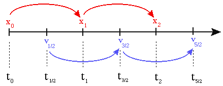
We can do the same thing to equation (3) above:
The equation here is a bit more complex, but perfectly good for a fully explicit numerical integration of equation (1).
Python program
The Python program for the integration of the harmonic oscillator equation (1), using the leapfrog equations (5) and (6) is harmonic_oscillator_leapfrog.py. To make things simple, I use \(m = 1\) and \(k = 1\). We go through it now.
For the moment, we work without a force, i.e., \(F = 0\). As you see below, integration is fairly simple:
     from pylab import *

     ###############################################################################
     N = 10000
     t = linspace(0,300,N)
     dt = t[1] - t[0]

     ###############################################################################
     # integration function
     def integrate(F,x0,v0,gamma):
          ###########################################################################
          # arrays are allocated and filled with zeros
          x = zeros(N)
          v = zeros(N)
          E = zeros(N)

          ###########################################################################
          # initial conditions
          x[0] = x0
          v[0] = v0

          ###########################################################################
          # integration
          fac1 = 1.0 - 0.5*gamma*dt
          fac2 = 1.0/(1.0 + 0.5*gamma*dt)

          for i in range(N-1):
               v[i + 1] = fac1*fac2*v[i] - fac2*dt*x[i] + fac2*dt*F[i]
               x[i + 1] = x[i] + dt*v[i + 1]
               E[i] += 0.5*(x[i]**2 + ((v[i] + v[i+1])/2.0)**2)

          E[-1] = 0.5*(x[-1]**2 + v[-1]**2)

          ###########################################################################
          # return solution
          return x,v,E
This piece of code actually doesn't solve anything, yet. I created the function "integrate(F,x0,v0,gamma)", to make it easy solving the problem with different parameters and compare them. For example:
     ###############################################################################
     # numerical integration
     F = zeros(N)
     x1,v1,E1 = integrate(F,0.0,1.0,0.0) # x0 = 0.0, v0 = 1.0, gamma = 0.0
     x2,v2,E2 = integrate(F,0.0,1.0,0.05) # x0 = 0.0, v0 = 1.0, gamma = 0.01
     x3,v3,E3 = integrate(F,0.0,1.0,0.4) # x0 = 0.0, v0 = 1.0, gamma = 0.5
When plotted, it gives (see code for details):
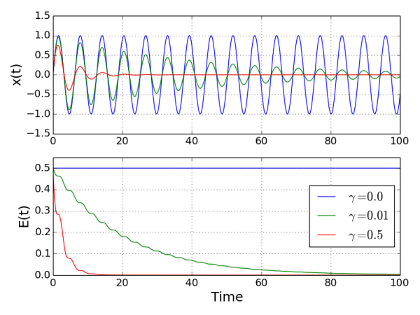
So we see that without damping (\(\gamma = 0\)), energy is conserved. With damping (\(\gamma \neq 0\)), the energy drops, faster for a higher value of \(\gamma\), as expected. The oscillations in the energy might look weird but think about it a moment. Energy loss is associated with the damping force, proportional to \(v\). If \(v\) oscillates, there is periodically a certain time lapse where it is zero or close to it. In this interval of time, damping is absent and energy is constant.
To add a driving force, I recycle the function packet() from the Fast Fourier transform article, that I renamed force() to fit in the actual context:
     def force(f0,t,w,T):
          return f0*cos(w*t)*exp(-t**2/T**2)
Then I tried three cases were forces had the same amplitude and duration, but with different frequencies: \(\omega_0\), 0.9\(\omega_0\), and 0.8\(\omega_0\), \(\omega\):
     F1 = zeros(N)
     F2 = zeros(N)
     F3 = zeros(N)
     for i in range(N-1):
          F1[i] = force(1.0,t[i] - 20.0,1.0,10.0)
          F2[i] = force(1.0,t[i] - 20.0,0.9,10.0)
          F3[i] = force(1.0,t[i] - 20.0,0.8,10.0)

     x1,v1,E1 = integrate(F1,0.0,0.0,0.0)
     x2,v2,E2 = integrate(F2,0.0,0.0,0.0)
     x3,v3,E3 = integrate(F3,0.0,0.0,0.0)
It gives (see code for details):
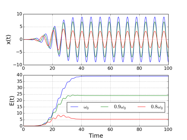
So we see that an oscillator driven close to its natural frequency \(\omega_0\) gains energy from the driving force, as expected. Damping was neglected (\(\gamma = 0\)). If we add it and drive three different oscillators with the same force:
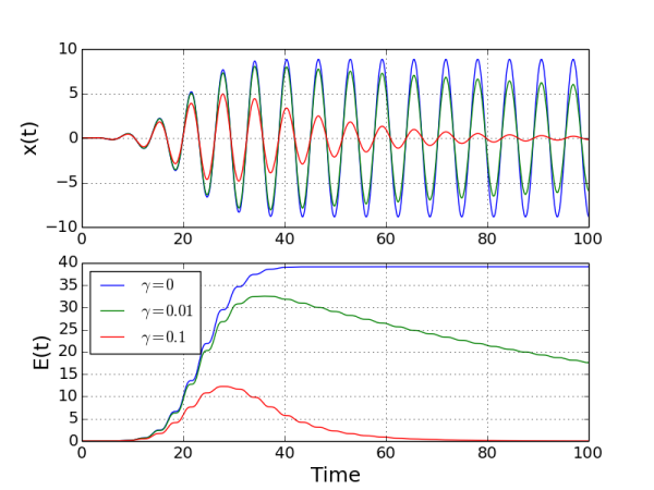
     x1,v1,E1 = integrate(F1,0.0,0.0,0.0)
     x2,v2,E2 = integrate(F1,0.0,0.0,0.01)
     x3,v3,E3 = integrate(F1,0.0,0.0,0.1)
then you see, below, that the oscillators gain energy, but also loose some due to damping. When damping is strong, energy is lost almost immediately after the driving force stops.
Well it happens that the driven harmonic oscillator (with damping) is a simple equation that is widely used to model how light interacts with atoms see this reference, for example. I even got myself interested on improvements to reproduce some quantum mechanical behaviors of atoms in strong light fields for modeling nonlinear optics (see here).
I let you now explore with your new tool.