As a first article in the CSSG series, I deal with the Fast Fourier Transform (FFT), in Python. In particular, I propose the simple example of a Gaussian wavepacket, whose analytical transform is known, to deduce the right normalization factor.
Python and the fast Fourier transform
The FFT is a special category of algorithms developed to compute the mathematical Fourier transform very quickly. We will not go into the details of the algorithm itself, but simply see how to use it, in Python. If you want to know more about how FFT works, see the Wikipedia article.
For example, if you have a time series \(E(t)\), you have access to its angular frequency content through the Fourier integral transform:
where \(i = \sqrt{-1}\). There is also the inverse Fourier transform:
The FFT computes a discrete form of the Fourier transform, i.e., it approximates the integral by a sum. For example
you see immediately that there is a \(dt/\sqrt{2\pi}\) missing. It must be added explicitly.
In Python, FFT functions are available in the scipy.fftpack module. You can import the functions you need by adding, for example, the following call to your Python script
from scipy.fftpack import fft,ftshift,ifft,ifftshift
This is what we will need later. But in the program I propose, it is automatically called by
from pylab import *
Fourier transform of a Gaussian wavepacket
The Gaussian wavepacket is common in physics and chemistry. It is characterized by a function similar to this one:
In complex notation:
The calculation of its Fourier transform is a bit lengthy so I give the final result only:
In a moment, we will look at the spectral density
This is the equation we will compare with the numerical Fourier transform, in a moment.
Python program
First of all, the Python program described below: python_fast_fourier_transform.py. We now explain what it does.
The purpose of the following program is to perform the numerical Fourier transform of \(E(t)\), compute the power spectral density, and compare against the analytical form given above.
First, it is convenient to define the following two functions that were defined earlier:
 def packet(E0,t,w0,T):
      return E0*cos(w0*t)*exp(-t**2/T**2)

 def packet_spectrum(E0,w,w0,T):
      return (E0*T/(2.0*sqrt(2.0)))**2*(exp(-(w - w0)**2*T**2/4.0) + exp(-(w + w0)**2*T**2/4.0))**2
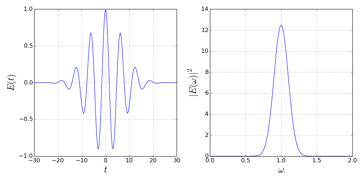
Then, we can readily see what the analytical signal and its spectrum looks like with the following piece of code:
 from pylab import *
 rcParams['axes.grid'] = True
 rcParams['font.size'] = 14
 rcParams['axes.labelsize'] = 22

 E0 = 1.0
 w0 = 1.0
 T = 10.0

 ###############################################################################
 # time axis
 n = 800
 t = linspace(-150,150,n)
 dt = t[1] - t[0]

 ###############################################################################
 # angular frequency axis
 dw = 2.0*pi/(t[-1] - t[0])
 w = arange(-n/2,n/2)*dw

 ###############################################################################
 figure(figsize=figaspect(0.5))

 # time series
 subplot(121)
 plot(t, packet(E0,t,w0,T))
 xlabel(r"$t$")
 ylabel(r"$E(t)$")
 xlim(-30,30)

 # spectrum
 subplot(122)
 plot(w, packet_spectrum(E0,w,w0,T),'-',label='analytical')
 xlim(0,2)
 xlabel(r"$\omega$")
 ylabel(r"$|E(\omega)|^2$")

 tight_layout()
 show()
that gives
The fast fourier transform of the analytical wave packet is done by calling fft(), combined with fftshift(). The shift function is necessary to order the data array in the correct way. For example, the following lines
 signal = packet(E0,t,w0,T)
 trans = fftshift(fft(signal))*dt/sqrt(2.0*pi)
 num_spec = abs(trans)**2
give a spectrum that can be compared directly with packet_spectrum() [note the dt/sqrt(2.0*pi)]:
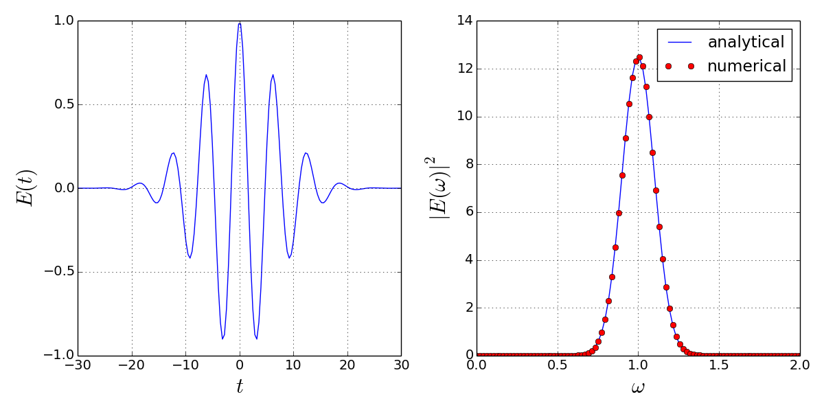
So it fits.
For the inverse Fourier transform, the normalization factor is slightly different:
inv_trans = ifft(ifftshift(trans))*dw/sqrt(2.0*pi)*n
Note the 'n' at the end. It is specific to the SciPy implementation of the FFT. Also, dw is used instead of dt because the inverse Fourier transform is an integral over the angular frequency. Finally, see that ifft() and ifftshift() are called, where the 'i' stands for 'inverse'.
All that said, we can compare inv_trans to the initial signal:
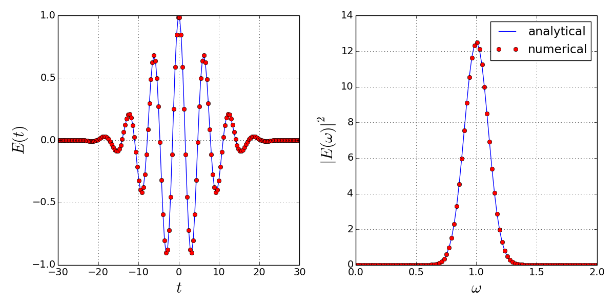
And we see again that it fits.
Summing up, we have seen how to perform fast Fourier transforms in Python, with the help of the fftpack module of the SciPy library. Most importantly, we have seen how to normalize the transform and the inverse transform to obtain results that are numerically correct.